July 16, 2018
Recurse Center - First steps w/ Queues
I am currently attending Recurse Center in New York City, where Im studying discrete event simulation & queueing theory for the next 12 weeks. I plan to study and gain intuition about queueing theory by working through Mor Harchol-Balters "Performance Modeling and the Design of Computer Systems" textbook and through simulation, playing with knobs and asking what if questions about scenarios in the book and from outside experience. What are the boundaries of the universe of parameters and what happens at the edges?
A queue is the summation of the difference between an arrival process and a service process. A queue can appear anytime an arrival rate is higher than a service rate at a point - a short-term difference leads to a transient queue, a long-term difference leads to a standing or unbounded queue.
Imagine a road - draw a box around a stretch of the road. A fixed n cars/sec arrive at the box, a service process allows n cars/sec to leave. No queue forms, the time it takes for a single car, its service time, is only governed by its speed and the size of the box.
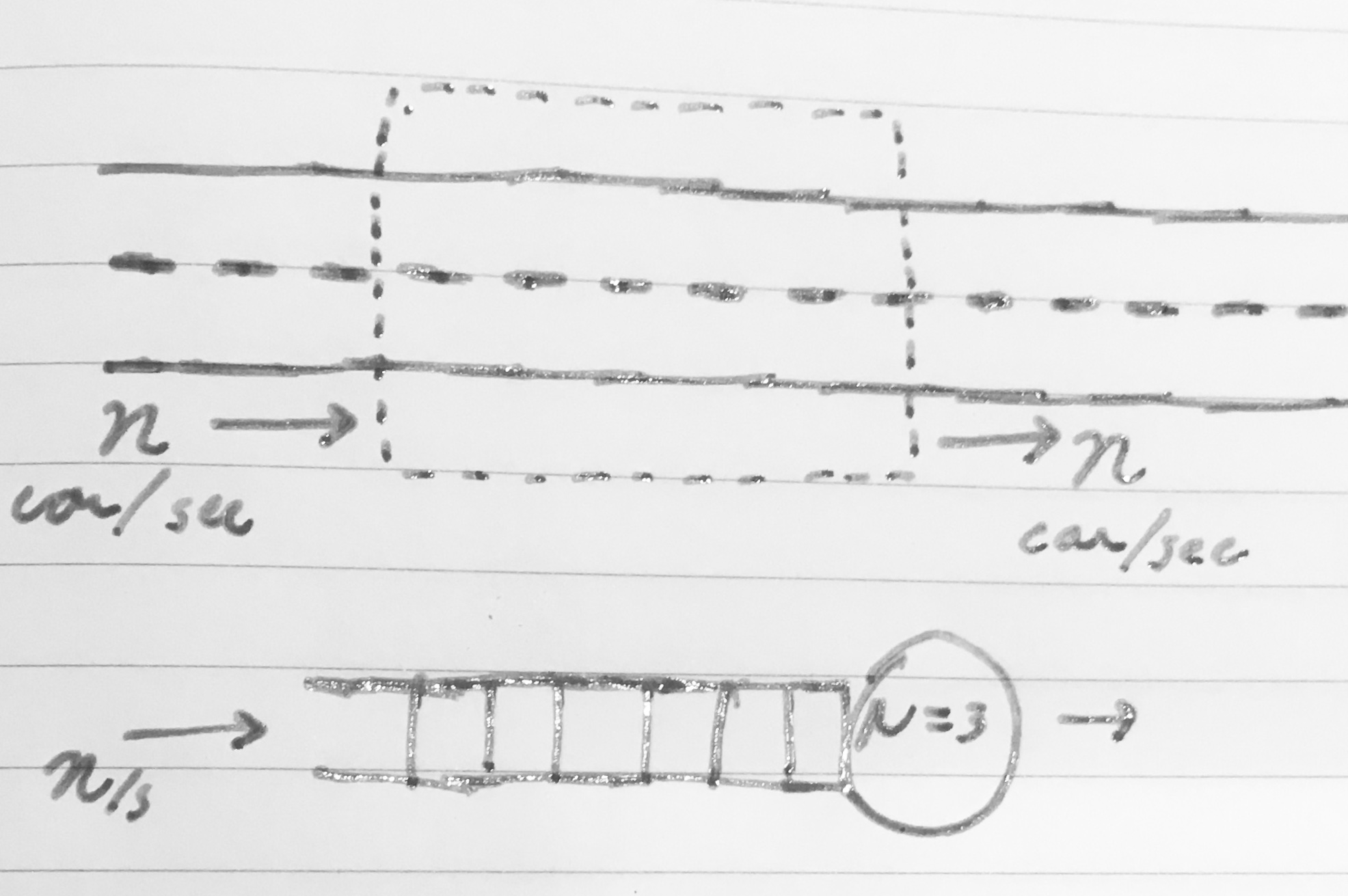
Now imagine a row of ducklings wanders across the eastbound lane.
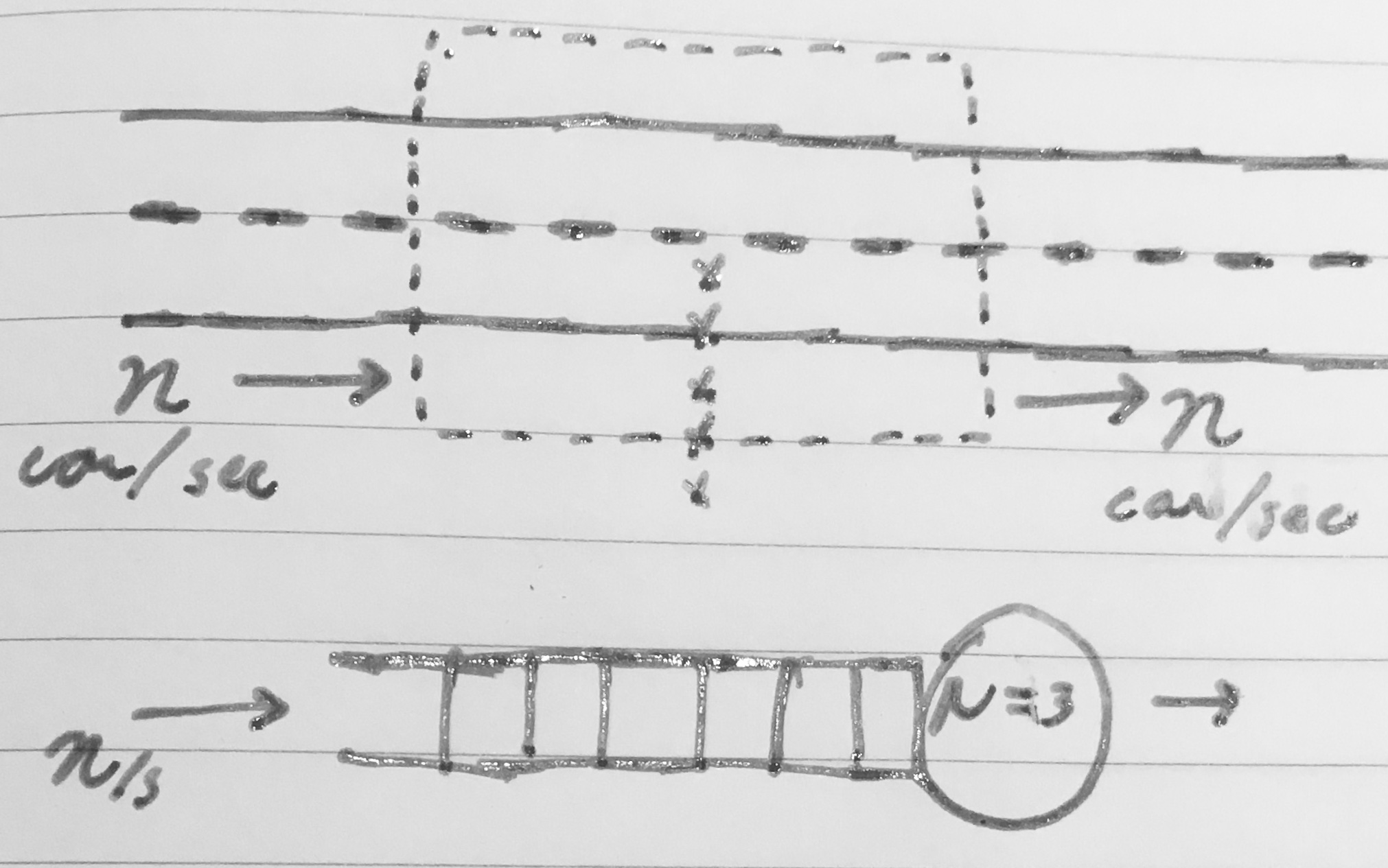
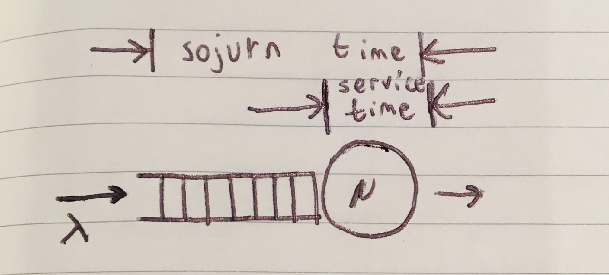
The maximum service rate transiently drops and cars queue to wait patiently for the ducklings to cross. The sojurn time, the time from when a car arrives at the box until it leaves, rises to include time spent waiting.
Schematically, queueing systems are represented by interconnections of queues, processors, and switches. The road example would be -
Queueing theory seeks to understand how queues form, behave, and how they should be controlled. Queueing theory also seeks to understand and control how units of work flow and wait in systems and to maximize throughputs or minimize average/worst-case delays.
Queueing theory generally assumes a systems long-term arrival rate is less than the long-term service rate - otherwise a system would diverge and queues could grow without bound.
Queueing theory allows arrival and service processes to be statistical counting processes - for example, on average λ units of work/sec may arrive, but the arrivals may not be uniformly spaced in time and the inter-arrival time may follow many distributions. Units of work may also take non-uniform resources/time to service, again following some distribution.
Tero Parviainen (@teropa) wrote a fantastic interactive tool to experiment with Markov arrival processes, a common arrival process where inter-arrival times are independent - A Dash of Queueing Theory. It is worth spending some time looking at both the cumulative arrival and service processes in his examples - it is important to understand that queues can form even when average arrival and service rates are matched.
Via queueing theory, we can approach questions like - "Should we have one processor with a service rate of μ or have multiple processors N, each with a service rate μ/N?" or "When should we power on/power off additional processors to service work?" or even "When/how should a queue push back on a source to change an arrival process?"
Some of these questions may have other approaches - control theoretic approaches to when to power on/off additional processors using the first derivative of queue depth have been fruitful, for example.
Mor Harchol-Balters text starts with a few design questions - Id like to highlight two:
-
Imagine a system where work arrives at a server, following a Markov process (inter-arrival times follow exponential distribution, memoryless process); on average, 3 units of work arrive each second. The server is able to service up 5 to units/sec.
Imagine the arrival rate doubles; how much faster do you need to make the server to maintain the average sojurn time?
It turns out that the server needs to get less than twice as fast to maintain the average sojurn time! I found this result fairly counterintuitive.
I wrote a simple discrete event simulator to work through this scenario, in two steps. First I started with a system where 3 units/sec arrived following a Markov process and 4 units/sec could depart. Then I turned up the service rate from 4 units/sec -> 8 units/sec; the distribution of sojurn times shifted:
This is a stacked violin plot of the 3 units/sec // 4 units/sec scenario (blue) and the 2 units/sec // 8 units/sec scenario (orange). In a violin plot, the width of a horizontal slice represents the part of the Density Function that is at a particular y-axis value. The means and extrema are highlighted by horizontal bars.
In both the blue and orange violins, we see most of of the PDF at zero sojurn time (no delay). The blue distribution has substantial density at 1 and 2 units of delay, whereas the orange (faster server) distribution does not. The mean of the orange distribution is just a hair above zero; doubling the service rate has more than halved the average sojurn time.
Lets now double the arrival rate as well, from 3 units/sec -> 6 units/sec:
The blue distribution is the same as the prior plot - 3 units/sec arrive, 4 units/sec service rate.
The orange distribution is for 6 units/sec arriving, 8 units/sec service rate. The Density Function of the faster servers sojurn time remains better than the original scenario!
Looking at the time series of sojurn times of the initial case (3 units/sec // 4 units/sec) was crucial to understanding this result.
Here the x-axis is job sequence #, the y axis is sojurn time.
There is underlying structure here! If job N experiences a delay, it is more likely that job N + 1 experiences a delay. Intuitively, the system is stateful - a job can see a unloaded or loaded system, based on recent history.
Doubling the service rate halves the amount of time required for a single job to be processed; it also reduces the probability that a job will see the system in a bad state.
Combining the two effects more than halves the average sojurn time.
(6 units/sec // 8 units/sec scenario - the x scale is different from above because a higher arrival rate results in more jobs arriving within a given time)
-
Imagine a system where work arrives following a Markov process. You can feed this work into either one server with a service rate μ or into N servers with a service rate of μ/N. Under what circumstances would you choose one server or N servers?
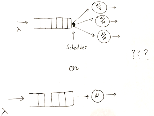
Let us start with the assumption that there is sufficient work to fully utilize all N servers; if there is insufficient work, one server would be preferable - the multi-server configuration would have idle capacity.
The result is it depends on the variance of the job size distribution - High variance favors multiple slower ones servers over one fast server.
Lets start with the simple case where there is zero variance in job size - in this case, the fast server will finish a job every 1/μ seconds, the slow servers will finish N jobs every N/μ seconds. Both configurations should perform identically.
In the high variance case, however, we can end up with an expensive job in front of a cheap job - a classic head of line blocking scenario. The one server configuration will force the cheap job to wait for the expensive job whereas the N server configuration would allow the cheap job to slip around the expensive job.
We will come back to this configuration in future examples.
Thank you to many peers at the Recurse Center for reviewing this post
Posted by vsrinivas at July 16, 2018 06:17 AM